Welcome!
One of my favorite pastimes is to just talk and talk about path tracing theory, and this is a great place for me to do that!
The goal fo this post is to ser as a intuitive guide to modern advanced global illumination algorithms. I see it as a resource for those wishing to naviagte the sometimes confusing intuition of advanced GI algorithms, and who want to understand the mathematical significance of these techniques and what makes them different. Specifically, it focuses a lot on what exactly path sampling techniques like vertex connections and photon mapping are doing, both on an implementation level, and on a theoretical, rigorous mathematical level, to truly convince you that these algorithms truly are amazing.
I will borrow from everyone’s favorite math youtuber 3Blue1Brown in that my goal is for you to feel like you could have discovered these algorithms yourself, and understand the motivations for their inception and modern-day usage. Above all, I want these algorithms to make sense, and to get people excited about them.
I will assume some basic familarity with Path Tracing, on the introductory level. You should know generally how a Naive Path Tracer works, and how BSDFs work. Here are some terms that may be a little confusing, though:
Dirac Delta Distribution (also called a delta distribution, a specular material, or describing a deterministic material)
A Dirac delta distribution is a mathematical object, representing distributions that integrate to a number but are zero on the entire domain except for one point, but in rendering it is most useful as a way to describe deterministic scattering in the language of importance sampling. Consider a perfect mirror: given an incoming direction, there is exactly one outgoing direction that contributes. All other directions have zero density. Rather than sampling from a continuous distribution, the material deterministically maps one direction to another.
In the application of path tracing, delta distributions are not necessarily very hard to intuitively think about. However, the specific ways that they interact with the actual mathematical foundations behind path tracing are honestly quite specific and hard to think about, so I will only explain up to the surface level, rendering engineer level understanding of them. (I wouldn’t be too comfortable teaching any more in depth)
Random Walk
Formally, a random walk describes traversal on a graph. In path tracing, it is a useful way to think about how light paths are constructed: each surface intersection is a vertex, and each scattering event chooses the next edge. However, graph theory has little to nothing to do with the techniques described here, so it serves merely as a useful corollary. In fact (fun fact!) it could be strongly argued that using graph theory at all to describe path tracing is not really rigorous either! You will see in the light transport equation section below (a subsection of Next Event Estimation) that the real, real light transport equation represents the integration domain in a really cool way that graph theory does not at all capture!
Importance Sampling and Monte Carlo Integration 🔗
Before we begin discussing actual techniques for estimating light transport, let’s review the basics of the problem at hand, and the tools we use to build our algorithms.
At its core, light transport is governed by an integral called the light transport equation, which can look something like this.
$$L_o(p, \omega_o) = L_e(p, \omega_o) + \int_{\mathcal{H}^2} f_r(p, \omega_i, \omega_o) L_i(p, \omega_i) \cos\theta_i , d\omega_i$$
This is James Kajiya’s famous light transport equation, which was used for many years (and still to today) to teach introductory light transport theory. Don’t get too attatched to it, though, because there is a better light transport equation that will be introduced soon. I won’t get into the specifics of this equation; all you need to know is that there is some integral that we are trying to estimate the value of.
It’s pretty easy to see why solving this integral analytically is impossible. However, we are able to calculate the function at discrete points, in a way. Therefore, we use a technique called Monte Carlo Integration, where we produce an estimator for an integral by probing the function at discrete points. What do we mean by points though?
As the name suggests, Path Tracing involves tracing paths of light. In practice, constructing a “point” of the integration domain to evaluate the function at consists of tracing connections between vertices in the scene that bounce from surface to surface, constructing a path connected by vertices. Hence, this is what is generally referred to as a random walk around the scene.
How do you construct this random walk then? Let’s consider the Kajiya equation for a moment: it is defined recursively, and at each step of the recursion, it integrates over the hemisphere around a surface. For an implementation, this translates to randomly picking a direction in the hemisphere to continue the random walk at each step of the recursion. However, this is not very efficient. For example, consider an interaction where you are processing the integral at a glossy surface. We know that for a given incoming light direction, glossy surfaces generally reflect a lot of light in one specific direction, and not so much in other directions. By uniformly randomly picking a direction to continue the random walk, you will usually pick a direction that is not very strongly favored by the physical behavior of the material (it’s not usually close to the perfect reflection direction). The solution, then, is to weigh your sampled directions according to how light actually behaves when hitting that surface. This means, for a glossy material, sending random walks towards the direction where the light usually goes. In a more extreme case, for dirac delta surfaces, for a given incoming direction there is only one specific direction that any light actually leaves in, so no uniformly random sampling of the hemisphere will ever produce a path that carrys any light.
Another way to think about this is creating physically plausible paths, not just arbitrary paths. This is because physically plausible paths have much more contribution than any arbitrary path! Taking a step back, this process is essentially biasing how you pick samples to feed your Monte Carlo Estimator, which is a problem, since bias is bad! In order to unbias it, you divide the contribution of that sample by the probability (the pdf) of choosing that sample. This makes sense, since if you divide a sample that was very likely by its pdf (a relatively large pdf), its contribution is smaller, correcting for the fact that you will generate that sample with high probability. On the other hand, a rare sample will have its contribution boosted by dividing by its small pdf, making up for the fact that it is only rarely generated. A way to think about this is just that you are choosing to take shortcuts and biased techniques that allow you to use less computation to get a better result, but because you are doing all these tricks, you need to be accountable for how much that biased the result, in order to unbias the result at the end. This process is called Importance Sampling, and it is how we make path tracing computationally feasible, via choosing the paths that we feed into our estimate more physically plausible, and thus more likely to carry a large amount of path contribution (light), while keeping the final result unbiased.
In the following sections, I will write extensively on pdfs of sampling directions and pdfs of entire path contributions. Every single light transport algorithm requires the creation of some sort of random walk, which will always require importance sampling pdfs, and those pdfs are exactly these importance sampling pdfs. For some additional context: Any time you generate a sample (like a point in the integration domain) that you will probe the integration function at, for each step you took to generate it (importance sampling), you need to multiply the pdfs of those sampling events together as a sort of record keeper to keep you accountable for the shortcuts you took.
Naive Path Tracing 🔗
Naive Path Tracing is the strategy where the integrator follows a random walk that originates at the camera as it traverses the scene, and only adds a contribution to the image if the random walk happens to land on a light. Clearly, if lights are small, this strategy will be horrible at rendering a smooth looking image due to the sheer difficulty of randomly scattering into a light source. The core problem with this strategy is that you only gain a few light contributions per random walk because you rely on the chance of randomly finding a light. In other words, the ratio of random walks to samples generated is very unoptimal, especially considering that random walks, and the intersection tests that they require, are easily the most expensive part of path tracing. To optimize, one might look to shift this ratio to be more favorable, motivating the use of techniques like Next Event Estimation.
Next Event Estimation 🔗
Next Event Estimation, also called direct light sampling, answers the problem of Naive Path Tracing by proactively searching for useful samples instead of relying on random chance to find them. Intuitively, if I have a point that is next to a lightbulb, clearly some light is going to arrive from the light to the point, as long as there is no object blocking the line of sight from point to light. From an implementation perspective, this means that you are drawing a shadow ray (test for occlusion) from a point on your camera path, directly to a light in your scene. It’s an incredibly simple and intuitive way to find light in the scene, which is why it predates path tracing as a whole.
Short tangent: The light transport equation(s) and integration domains 🔗
Once you get around to implementing Next Event Estimation, there is one specific step that is very confusing when you first get to it. NEE is performed, usually, by randomly choosing a point on a light in the scene and attempting a connection to it. Therefore, your sampling PDF is evaluated in inverse area (e.g., $1/\text{Area}$). Wait, what? That should feel kind of weird. If you are familiar with the PDFs generated during the random walk, you would remember that those PDFs are all generated by sampling a hemisphere around the surface. It feels weird to just say 1/area! And you would be right to think that. Recall the Kajiya light transport equation:
$$L_o(p, \omega_o) = L_e(p, \omega_o) + \int_{\mathcal{H}^2} f_r(p, \omega_i, \omega_o) L_i(p, \omega_i) \cos\theta_i , d\omega_i$$
This integral recursively defines the radiance at a point via integration over the hemisphere around that point, in solid angle measure ($d\omega_i$). This is why the BSDF PDFs used in traditional path tracing look the way they do. It’s to natively fit this integral! But then, how do you justify doing NEE? How does an area-based PDF fit into a solid-angle integral?
The answer is a standard calculus change of variables. You don’t actually switch domains or evaluate two different integrals; instead, you mathematically transform the integration domain of Kajiya’s equation from the local solid angle of the hemisphere to the surface area of the light sources. By applying the Jacobian determinant (essentially the geometry term), you build a bridge that perfectly adapts your area-sampled light point into the solid-angle equation.
However, while Kajiya’s recursive model can handle standard path tracing and NEE via domain changes, it is admittedly a little awkward. First of all, Kajiya’s equation is a little stiff: it lays out every term you need to consider at its most basic level, which despite making it much more implementation friendly, essentially locks any use of it to standard unidirectional path tracing. It is very clear to see that its not just built for unidirectional naive path tracing, it IS unidirectional naive path tracing. The whole charade we had to go through to incorporate next event estimation, essentially changing or cancelling out almost all of the terms in the equation, is awkward. While its a useful tool for making your first physically based path tracer, it will not and cannot help you with understanding more advanced forms of light transport.
For a more universal mathematical model that elegantly supports these advanced algorithms, look no further than the formulation made by Eric Veach:
$$I_j = \int_{\mathcal{P}} f_j(\bar{x}) , d\mu(\bar{x})$$
Here, instead of integrating over solid angle at one point in a recursive manner, this integral evaluates the full path space of the scene. Formally, the scene is defined by a surface manifold $\mathcal{M}$ (the collection of all surfaces in your scene). A single path $\bar{x}$ is a point in the product manifold:
$$\mathcal{P} = \bigcup_{k=1}^{\infty} \mathcal{M}^{k+1}$$
This means the integration domain is the union of all possible Cartesian products of the manifold $\mathcal{M}$ with itself. A path is just a single point $(x_0, x_1, \dots, x_k)$ in this high-dimensional space.
The beauty of this is in how general its integration domain is. By defining the problem over the space of all possible paths in area measure, it creates a neutral ground. Any sampling technique you want to use-whether bouncing rays by solid angle or picking points by area-can be mapped into it. However, clearly, this integral is a lot less immediately helpful, as most of the terms that actually are needed for implementation are included in the very complicated $f_j(\bar{x})$ term. However, its universality lends itself to more flexible ways to think about and interpret light transport.
The big conceptual shift is that in Veach’s integral, your master measure is surface area. This means that when you are following this integral, you won’t be converting your NEE PDF to solid angle; you will be converting your BSDF PDFs to area measure! This means that when calculating the path contribution $f_j(\bar{x})$, every segment on your path contributes a new geometry term to fit this area measure, which one would think complicates the math. But here is the brilliant trick of the math: the physical Geometry term of the path perfectly cancels out with the Jacobian of the solid-angle PDF’s used to generate the path. This cancellation is why your standard random-walk throughput code remains entirely unchanged when shifting perspectives.
This makes sense intuitively, since both integrals are describing the same physical phenomenon, the only difference is how they choose to parameterize the integration domain. It makes sense that the path contribution calculated using the same sampling techniques would provide the same contribution whether you measured using a solid angle ruler, or a path product manifold ruler. The Monte Carlo estimator is invariant to the domain. Veach simply unrolled Kajiya’s local equation into a global area space, giving us the universal coordinate system required to fairly compare any sampling technique we can dream up.
Sub-Tangent: (Integration) Domain Expansion (extension) 🔗
Veach’s light transport equation is geared towards traditional surface based light transport. That is-it considers paths made up of points on surfaces. In practice, this acts under the assumption that light travels in a straight line through non-surfaces and only changes direction when it hits something, which is mostly true at a macro level. However, many phenomena that one may wish to render happen to break this assumption, at least in a practical sense. The easiest one to see is practical rendering of volumetrics.
While physically, the surface integral can technically describe volumetrics by modeling all the tiny particles that are part of a volume as their physical reality, it is easy to see how this is computationally impossible. Thus, it is needed to extend/expand the domain to not only include interactions on surfaces, but between surfaces where a volume may exist. For example, if a beam of light scattered off of a wall, went through some smoke, and hit another wall. You can’t just only consider the two wall hits because going through the smoke did in fact change the light in a meaningful way. This motivates an extension of path space that includes any volumetric interactions, such as one that considers points not on a surface manifold per se, but in free floating space as well.
Another extension of path space is the lobe-based extension of path space. In the real time rendering algorithm ReSTIR PT, the authors needed a way to keep track of the state of existing paths, for reasons out of the scope of this section. Part of this record keeping was the need to keep track of which specific lobe of a bsdf a path interacted with, in order to scatter to its next point. Therefore, they extended the path space domain to give each point in a path a lobe index that indicated whether that path sampled, for example, the clear dielectric coat on the top of the material, or the diffuse middle layer, or even a subsurface scattering bottom layer.
The key realization here is that this does not invalidate, or even meaningfully change the light transport physics and math, since this is just another way to parameterize the integral. And additionally, it was not motivated by a need to model additional phenomena, it was literally just added to make an algorithm easier to describe. This should help contextualize what kind of problem path tracing is. You can imagine that there is some theory of everything integral and integration domain that can be used to describe anything you want to render, but to make things computationally feasible, we take simplifications of that problem based on what our goal is. If there are no participating media (volumes), then we can consider a surface only parameterization. If we don’t care too much about reconstructing path connections based on the lobe sampled, we don’t need ReSTIR PT’s domain extension.
What this means for Kajiya and Veach, then, is that neither truly describes the problem at hand. However, Veach’s (and similar cartesian product type definitions) is able to balance flexibility and practicality, by being more general and yet still being specific enough to allow for scientists to work around, as well as being, as I believe, the most intuitive way to think about path tracing. After all, we are tracing paths, not points on a hemisphere!
Tangent over!
NEE is efficient because at every bounce of its path, it is able to try and generate a valid light sample at every intersection. Additionally, since it forces a connection to a light source, it doesn’t care how small the light source is. It renders small lights just as (if not more) efficiently than large lights. It is not without problems though, namely that its not able to resolve direct viewing of light sources at all! I can see the light emitted by a lightbulb, but I can’t see the lightbulb itself! Interestingly, this is exactly what Naive Path Tracing excels at. If only there was a way to combine them…
Multiple Importance Sampling 🔗
Multiple Importance Sampling (MIS) (Veach and Guibas 1995) is a framework for combining the contributions of multiple sampling strategies in a smart and efficient way. To understand how it works, we can look at how it manifests in combining NEE with Naive Path Tracing. Theoretically, both of these strategies, when done on their own, create a perfectly energy conserving image (even if some parts are undersampled). However, as we have discussed, they each have their own weaknesses that the other excels in. Obviously, adding both of their contributions together would be wrong, since you are adding double the correct amount of light. What if you add 50% of the NEE contribution and 50% of the Naive contribution? That would be technically energy conserving, but it still won’t look right, your light sources will be darker because only half of your samples actually lit them, and if your light source is small you scene will only be about half as bright, since while nee handles its half well, Naive PT completely fails at filling its half. The solution is to use MIS to automatically balance how much each strategy contributes on a case by case basis, using something like this balance heuristic:
$$ w_i = \frac{p_i}{\sum_{k} p_k} $$
where $w_i$ is the weight for the ith strategy’s contribution, and $p_{i}$ is the probability of generating that specific sample. Note that this means that the weights for all strategies to generate a given sample should sum up to 1, making sure that we are conserving energy. Therefore, the weight for NEE would be equal to
$$ w_{nee} = \frac{p_{nee}}{p_{nee}+p_{naive}} $$
and likewise the weight for Naive PT would be:
$$ w_{naive} = \frac{p_{naive}}{p_{nee}+p_{naive}} $$
This means that every time you generate a sample with either strategy, you have to calculate the probability of having done it with the other strategy, and use that to generate a weight for the sample. If this strategy was very likely, it’ll take up more of that 1.0 total weight, and if it wasn’t very likely, then it’ll take up less. This way, your renderer will adaptively weight up or down the samples it generates to use the best of each strategy.
Note that, technically, the probability of doing each strategy is the FULL probability of traversing the random walk, times the probability of doing nee, or scattering to a light via random walk. It is because you are evaluating probabilities for the strategies at the same point that you can essentially cancel out the path history, and just compare the probabilities of sampling a light versus scattering to a light. This makes MIS pretty simple, and combined with the simplicity of the balance heuristic, the Naive PT + NEE using MIS integrator is basically standard for a easy integrator to write that is also incredibly robust.
It’s just a shame, though, that so many people will never get to experience to joy of doing MIS with an essnetially arbitrary amount of strategies that scales with how long your paths are, such as in Bidirectional Path Tracing!
Bidirectional Path Tracing 🔗
Bidirectional Path Tracing has two main goals. One is to increase the amount of samples per intersection test by aggressively reusing the paths you’ve generated, and the other is to explore parts of the path space that are hard or impossible to generate with unidirectional techniques. The first goal is easy to understand. The second goal, however, touches upon the real reason that BDPT is relevant in the first place. The problem with unidirectional path tracing is that by generating samples that always trace from the eye, you are ignoring a large section of the path space upon which you are integrating. One of the biggest examples of this is caustics.
Caustics are the phenomenon when light is focused by a material that acts near deteriminstically on incoming light that ends up focusing photons into specific shapes. Most famously caustics are seen when light passes through a refractive material like glass or water (dielectrics) and is focused into patterns due to the lensing effects of the dielectric. The problem with rendering caustics with unidirectional methods is that you are essentially trying to traverse backwards along a caustic path. To do so, you must hit the material on which the caustic is displayed, and scatter randomly towards the dielectric in the exact angle to refract through and hit a light. When rendering caustics, light sources are often very small and powerful, making hitting them backwards through a dielectric quite difficult. This is beginning to sound like the issues we encountered when first introducing Naive Path Tracing! Why are we waiting to scatter through the material and randomly hit a tiny light when we could just sample a light through the dielectric?
There are two main problems with that. One is that, as a rule, NEE cannot be performed from a deterministic (dirac delta) surface, such as a perfectly deterministic dielectric. It is because at a point on a dielectric, you can’t ask the question of, how much outgoing radiance is going in x direction, from the incoming photons from a visible light? The answer is zero, because it didn’t. By the nature of the delta distribution, there are two exact directions that the photons from the light could have traveled, the reflection direction and the refraction direction. The probability that photons were leaving in any other direction from the light is zero. You can’t say what-if, because it didn’t.
The other problem is that, you can’t perform NEE THROUGH a dielectric. Its easy to see how, if there is something between a surface and a light, you can’t rely on the direct visibility calculations, even if that something does let light through in some way. For the case where that something only attenuates light, you can actually modify your shadow ray function to track how much the shadow ray is attenuated, but since dielectrics actually bend the paths of light, you fundamentally cannot draw a straight line through the dielectric and say that is a path of visibility, because its not, and it never would be for a delta distribution.
There is however, a family of rendering techniques that circumvents this issue, including such techniques as Manifold Next Event Estimation (MNEE), and Specular Manifold Sampling (SMS) that uses root solvers to look for valid refractive paths through perfectly deterministic surfaces. However, currently the Novum Renderer does not current support those techniques.
Clearly, the existing Naive PT + NEE strategy won’t work for caustics, especially caustics from small lights. Its not that it cannot, its just that it is incredibly inefficient at doing so. The solution to this, is to simply trace not from the camera, but from the light itself, bringing us to Bidirectional Path Tracing, a technique that traces random walks from both the camera and from the light. These random walks are called the light and camera (or eye) subpaths, and they are made up of vertices. What makes BDPT good for resolving caustics is that random walking from the light very naturally resolves caustics. Since caustics are literally created from the focusing of photons, if you trace photons its natural that your paths get focused into certain areas of the scene, literally constructing the caustics as they were created in real life. If you were to trace a bunch of these light paths and store their locations, you may get something like this:
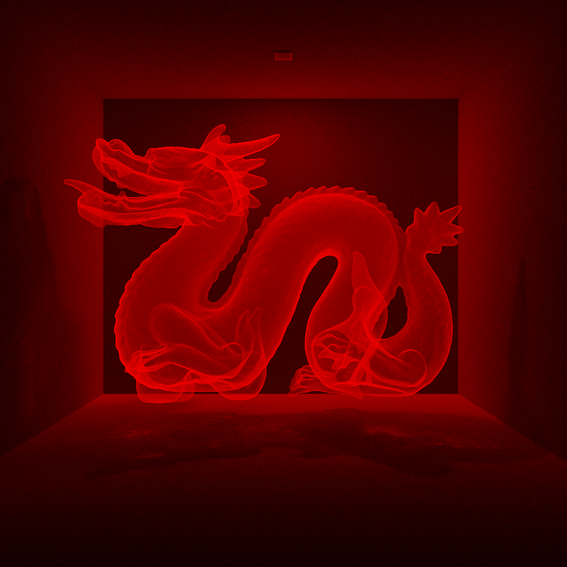 Heatmap of vertices on light subpaths in a scene with a dielectric dragon. Note the caustic patterns on the ground under the dragon.
The above image was made by just rasterizing the locations of light path vertices in a scene. Even though we can see the caustics now, we havn’t actually adapted them into our path tracing framework. Essentially, what good is tracing a bunch of light paths when we havn’t thought about how they actually link up to the camera? This leads us to the core of Bidirectional Path Tracing, the idea of connections.
Similarly to NEE, we can actually force connections between vertices on the light subpath and the camera subpath to form valid paths that connect the camera to a light source. In fact, ANY connection between ANY light vertex and ANY camera vertex forms a new theoretical path that could have linked the camera to the light.
The notation used for these paths uses the variables s and t, to denote the number of light and camera vertices, respectively. For example, s=2 and t=3 represents a connection between the 2nd light vertex and the 3rd camera vertex. You can have as many strategies for generating samples as the amount of pairs of s and t values, meaning that with 5 vertices in each subpath, you technically get 36 possible strategies (you can use 0 vertices as well!). This however comes with the caveat that some of the combinations, like s=0, t=0 don’t work, and others are ignored for other reasons.
Interestingly, something like s=0 and t=3, which uses no light vertices, is also a valid connection! In fact, this is exactly what Naive Path Tracing is! s=0, t=3 literally means the strategy where the eye random walk stops on the third eye vertex, which (for contributing samples) means that the random walk encountered a light by scattering randomly. In addition, because the first vertex of each path is defined to be on the surface of the light or on the camera itself, the strategy of s=1, t=3 is also just Next Event Estimation, since you are connecting a light’s contribution to a vertex on the camera random walk.
Having these two strategies already makes BDPT on par with the versatility of our unidirectional methods, but there is more! My favorite part of BDPT is something called Light Tracing. Light tracing is essentially the light path equivalent of doing NEE. Whenever t=1 and s>1 (sometimes s>=1 is used), you can connect a light subpath vertex directly to the camera. The logic is very similar to NEE, in that if we know that a photon landed in view of the camera, unless the surface is delta, there must be some radiance thrown towards the camera. Doing this with every vertex of a light subpath actually allows us to fully solve directly viewed caustics! The problem with this, though, is that since it can only render parts of an image where light path vertices are in direct view of the camera (and importantly non-delta surfaces!), it is inherently unable to render things like mirrors or specular dielectrics.
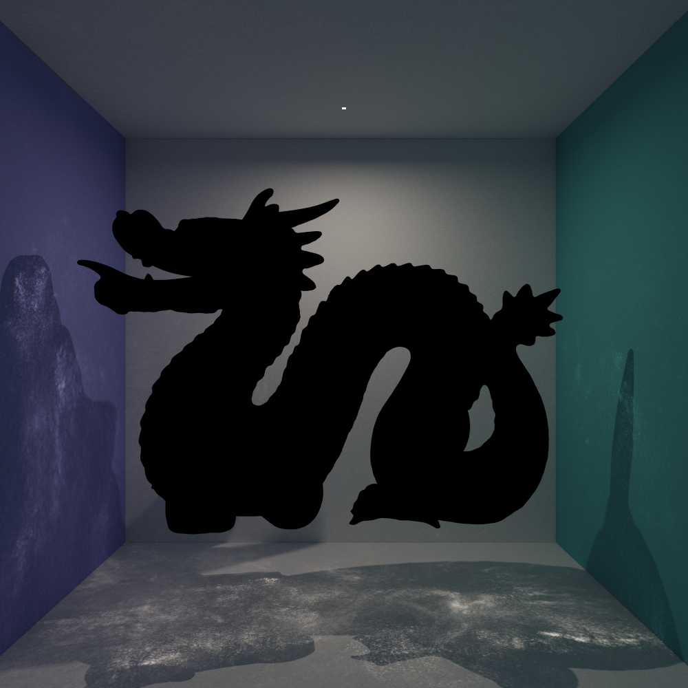 A dielectric dragon rendererd using only light tracing. Note that the dragon, which should be clear, is fully black.
Just as there is a light path analog for NEE, one might think that there is a light path analog for Naive Path Tracing, and there technically does exist such a thing. Just as one can wait for an camera path to randomly hit a light, one can also wait for a light path to randomly hit the camera. However, since cameras are normally never physically modeled with scene geometry, and since they are usually very small anyways, its just not really practical or neccesary to simulate this strategy, so it is almost always omitted.
What makes BDPT difficult, though, is Multiple Importance Sampling. While doing all of this subpath tracing and connections has given us a lot more ways to create samples, the truth is is that these strategies almost always overlap. For example, imagine a path from the camera to a light that is three segments long (it has four vertices). This path could have been created by an camera random walk that found the light by chance. It could also have been an eye random walk with 2 segments that filled the last segment by randomly sampling the light with NEE. It could have been a light subpath with 1 segment that connected to a camera subpath with 1 segment, etc etc. All of these constitute different strategies the same way that NEE and Naive PT constituted different strategies in our unidirectional path tracer, and as we discovered, different strategies need to be weighed together with Multiple Importance Sampling in order to be meaningfully combined. What makes it even worse is that this is just for one possible path construction. While we were connecting all of the path vertices on the two random walks, we were creating a bunch of different path shapes, each with their own possible ways of construction.
The difficulty with doing MIS in BDPT is that its very unrealistic to predict not only what the probabilities of the other strategies are, but even how many other strategies can be compared against. Doing so would require a processing of the entire path being constructed, which is very very implementation unfriendly due to the memory and computation overhead, since it would have to be done for each contribution generated, when each render pass can easily contribute 30+ contributions per pixel.
The solution to this is quite smart, actually, and is essentially what allows BDPT with MIS to be computationally feasible. This is absolutely the hardest part of BDPT, so bear with me!
The balance heuristic for a sample that could have been generated a large amount of ways appears like this:
$$ w_{1} = \frac{p_{1}}{p_{1}+p_{2}+p_{3}+p_{4}+…+p_{k}} $$
First, divide the top and bottom by $p_1$.
$$ w_{1} = \frac{1}{1+\frac{p_{2}}{p_{1}}+\frac{p_{3}}{p_{1}}+\frac{p_{4}}{p_{1}}+…+\frac{p_{k}}{p_{1}}} $$
Now, factor out a $\frac{p_{2}}{p_{1}}$ from all the terms in the denominator except for the 1.
$$ w_{1} = \frac{1}{1+\frac{p_{2}}{p_{1}}(1 + \frac{p_{3}}{p_{2}}+\frac{p_{4}}{p_{2}}+…+\frac{p_{k}}{p_{2}})} $$
Now, do the same for $\frac{p_{3}}{p_{2}}$, and repeat.
$$ w_{1} = \frac{1}{1+\frac{p_{2}}{p_{1}}(1 + \frac{p_{3}}{p_{2}}( 1+\frac{p_{4}}{p_{3}}(1 + …)))} $$
The point here is that the denominator of the weight can be split up into these components, mainly consisting of a ratio between path probabilities multiplied with the sum of 1.0, and an accumulated value that sums up the rest of the path contributions. To see why this form is so versatile, let’s look at what these probability ratios actually mean.
You may have noticed before that the majority of the sampling techniques that can generate a given path in BDPT are not the interesting NEE, or Naive PT, or Light Tracing strategies, but rather most of them are simply general connections between two intermediate vertices. The truth is that for each contribution generated, you are evaluating the contribution of a path that has one endpoint on the camera and one on the light, and while there may be five or ten or twenty possible ways to contruct such a path using general connections, you can only do NEE, naive path tracing, or light tracing one time each. Therefore, the recursively defined balance heuristic structure detailed above is simplified to clearly explain how these numerous general connections are weighed against each other.
The anatomy of a general connection can be broken down as follows. Just like NEE or a light trace connection, you are using the idea that if there is visibility between these two points, one which leads to a camera, and one which leads to a light, barring the case of determinstic (dirac delta) surfaces, there must be some radiance that goes from the light vertex to the camera vertex, or importance for the reverse case. As such, the probability for this connection itself is just 1. How do you find the probabilities for all the other possible connections though? What if you performed the connection one edge closer to the light, like connecting s+1 with t-1? What if you shifted it the other way to be one step closer to the camera?. These are both valid connections that could have produced the same contribution, and thus must be weighed accordingly. The recursive structure works by evaluating the weight by following this shifting of the connection edge, and since connections are always between a light and camera vertex, you must consider the probability of extending a light subpath to the previous camera vertex, or vice versa. In the short derivation above, the ratio of $\frac{p_{3}}{p_{2}}$ could represent something like the probability of a light vertex $y_1$ scattering back towards $y_0$ (as if extending the eye subpath), divided by the probability of $y_0$ scattering towards $y_1$ (as if extending the light subpath). The ratio of $\frac{p_{4}}{p_{3}}$ would thus just be the same thing, but shifted over an edge. You can see now, that these ratios are localized to just a single edge. As long as you know the local information surrounding one edge, you can calculate the ratio that can be used to build this recursive structure.
The shifting nature of how these ratios are build is very helpful when building the recursive weights, as well, since stepping forward is naturally corresponds to performing your random walk! Therefore, as you step forward in your random walk, you store an accumulated value of the structure $1 + \frac{p_{3}}{p_{2}}( 1+\frac{p_{4}}{p_{3}}(1 + …))$ (roughly) that essentially encodes the history of the path behind the current vertex, describing the probabilities of stepping forward and backwards along any of the edges before it (plus any other strategies used). Naturally, at a given edge you also need to add to this accumulated value, using the locally avalible data to construct the ratio that describes the probability of traversing the current edge, which will be delivered to the next vertex! It doesn’t need to know which strategy it will be used to calculate the weight for, because that can be handled by just multiplying a ratio into it, as shown above.
Regarding the non-general connection strategies, they are just inserted in the accumulation where they belong. If you are doing a light random walk for example, nee and naive path tracing happen at the first and second light vertices, so when you begin your random walk you just initalize the accumlated value with the nee and naive pt probabilities, and then wrap it in the recursive structure. That way, at connection time, the probability of doing nee or naive pt is weighed accordingly with the probability that the camera subpath extends all the way to the beginning of the light subpath, via all of those probability ratios (like it travels backwards along the light subpath). Also note that since a general connection needs to consider the strategies in the path history of both subpaths, the weight calculation uses both the accumulated values of the light subpath and the camera subpath.
If this was confusing, I do have another way of explaining why this might make sense. Before when we were doing the simple MIS with only two strategies, we simplified the balance heuristic by canceling out the path histories of the two strategies because they were equal (they took the same path to arrive to the current point). Formally though, each probability used in the heuristic is the FULL path probability representing all of the probabilities involved in generating that path in that way. Even if something like NEE is very likely, like if there was just one small light in the scene, if you are evaluating a connection super far away from the start of the light path, like s=30, t=10, doing NEE would correspond to the eye path extending 29 vertices backwards along the light subpath to then do that seemingly likely strategy. If you just used the nee probability by itself you would be vastly overestimating how likely it was, since it wasn’t weighed down by the probability of actually getting to the point where you could perform NEE. This is why its important that the nee probability, as you were accumulating your light path, is wrapped in all of those probability ratios that describe how likely it is to shift forwards and backwards along the path. Encoded in that recursive structure is the probability of stepping from s=30 to s=29, from s=29 to s=28, etc etc. This way, you can reconstruct the full probability of performing your strategies.
The beauty of this is that, at the cost of storing a few floats, you can evaluate the MIS weight in O(1) time, just by plugging these values into a formula alongside the current state. Even more importantly for GPU implementations, is that you only have to read this one (or two) value(s) from global memory. All the other values exist in your registers already!.
BDPT Implementation Details 🔗
Going from unidirectional methods to BDPT comes with one very big change for GPU implementations, and that is VRAM usage. Because you need to handle two random walks at the same time, and tracing both at once in one giant mega-megakernel would be incredibly harsh on register usage and very likely cause some memory spills, you have to store the state of at least one of the subpaths at all times. Since for each pixel, assuming one thread per pixel, you need to store the position, normal, incoming direction, throughput, cached mis terms, material information and flags (more if you are caching more detailed shading information), for each vertex. For larger images, the VRAM usage adds up very fast. Therefore, it is almost neccesary to use some sort of memory optimization in your path vertex structs. For example, using octahedral encoding to condense a 3 float normal or direction into a 32 bit unsigned integer is very helpful. Using half data types for throughput is also good as is packing flags and indices together into more unsigned integers.
It should also be mentioned that a theoretical understanding of BDPT and the actual implementation of it has a few very jarring differences. The biggest one is that you can’t always build the full probability ratio at every step, because you don’t actually have enough information to do so. Consider this situation: you are tracing a subpath and need to calculate the cached MIS term, meaning you need to find the probability ratio between scattering backwards towards the previous vertex and scattering forwards from the previous vertex to the current. The denominator probability is easy to find, its simply the pdf that took you to the current point on the random walk. However the numerator probability can’t be found yet. The numerator is supposed to be a BSDF scattering pdf evaluated at the current surface. You have the outgoing direction; it’s just the direction to the previous vertex, but you don’t have the incoming direction, since that depends on where the NEXT vertex is. Now, in an actual implementation it’s likely that you have already sampled an outgoing direction to continue your random walk in, and you may be tempted to use that as the incoming direction, but you have to remember that the cached mis value stored at the current vertex DOES NOT KNOW where the next vertex is. That is because when you use the cached mis value during connection, you are choosing where that next vertex is (wherever you decide to connect towards). The next vertex on the random walk is completely irrelevant.
Another very important detail with implementing BDPT is the need to perform extensive PDF unit conversions. BDPT was most famously formalized by Veach as a part of his path space integral, and it uses the form of that integral to its full extent. An implementation will require extensive use of jacobian terms to convert the units of BDSF sampling, as well as solid angle emission pdfs, into area measure to fit into the integral. This of course, is for the sake of comparing strategies with MIS.
Problems with Bidirectional Path Tracing 🔗
Earlier I mentioned that Bidirectional Path Tracing, through light tracing, solves directly visible caustics. It however, does not work for caustics that are NOT directly visible, such as caustics seen through glass, or caustics seen through a mirror. This is because of the existence of the Specular - Diffuse - Specular path segment (Specular roughly means a surface that acts generally determinstically). Imagine a situation where a path starts on a light, hits a the surface of some water in a pool, refracts into the water, hits the floor of the pool, and then hits the water surface again, refracting out of the water and hitting the camera. This could be expressed as LSDSE (L for light, S for specular, D for diffuse, E for eye). This is actually a pool caustic, the bands of light at the bottom of a pool, caused by light being focused by the disturbances in the water surface into patterns on the pool floor.
The problem is that Bidirectional Path Tracing has no way of rendering this! To understand why let’s explore our options. Our main strategy for resolving caustics, light tracing, won’t work because the diffuse vertex on the light path at the bottom of the pool doensn’t have visibility to the camera. We also cannot do light tracing from the vertex right before the camera since its on a deterministic surface. We can’t do any connections involving the caustic vertex because its surrounded by deterministic surfaces. One might be inclined to ask, well what if you considered instead the path LSDDSE, and did a general connection between the two diffuse underwater vertices. The problem here, is that the second diffuse bounce in that path essntially turns a bright caustic into indirect lighting. A caustic is only a caustic because you see at the original point, so these SDS paths are unavoidable, since they define what a pool caustic is. Another way of viewing this is that to approximate solutions to the rendering equation, you need to evenly sample the path space. BDPT and Unidrectional methods cannot sample paths that have SDS sections in them, and for a scene like a pool caustic, those paths make up a large amount of the most important and high contributing paths. the result is that a pool will just look unnaturally dark when there is a small powerful light (which creates the caustics), and it is rendered with BDPT or Unidirectional.
Its important to recognize, however, that just because BDPT isn’t good at rendering water, or caustics, doesn’t mean it isn’t a good algorithm. BDPT is good because it solves the inherent problem of finding light sources by making the light find the camera at the same time. This makes BDPT much better than Unidirectional methods at finding light when it is hidden, like when a light is physically hidden, such as a scene where you are seeing light come out of a keyhole.
Regardless, if you want to render good looking caustics that aren’t neccesarily directly visible, you will need another strategy.
Stochastic Progressive Photon Mapping 🔗
Stochastic Progressive Photon Mapping (SPPM) approaches the rendering equation from a different perspective than traditional path tracing. Traditionally, you try to solve the light transport equation by directly generating samples using Monte Carlo Integration to probe the radiance field at discrete points. However, SPPM, and photon mapping techniques in general, try to solve it by reconstructing an approximated version of the radiance field and integrating that using Monte Carlo Density Estimation.
Photon mapping, in general, is a multi-pass technique where you first shoot a bunch of photons and store where they hit your scene geometry. This is incredibly similar the storing light path vertices. The process of tracing the photons around the scene is exactly identical between the two, the only difference is in how they are managed and what data is stored. They are so similar, in fact, that earlier I lied in the BDPT section! The red image that I claimed mapped out the locations of light path vertices were actually the locations of photons stored in a photon map! Here it is again.
The truth is revealed! It's actually a photon map (even though its the same as painting light path vertices)After building the map, you perform a pass where you trace eye paths into the scene, and instead of bouncing them around, you only trace until you find your first surface that could possibly hold any photons (in practice this means the first non-specular surface), and perform a photon gathering step, where you query the photon map, and for each photon in a specific range, you add its contribution to the camera path. One of the coolest things about photon mapping is that since it works on density estimation, the intuition is very different from that of standard path tracing. One may be tempted to think of this photon gathering as connecting a light subpath to the camera subpath in a way. And remember, connections are always about what-ifs. However for this case, there is no what if! There is no way that you could reliably say what if the photon didn’t land where it did, and instead it landed directly on my eye vertex. Such a statement would be at best trying to articulate a connection between the previous position of that photon and the eye vertex, and at worst plainly nonsensical. What is actually happening is exactly what a density estimation is. By observing that in a radius around this point, there are some amount of photons sending radiance in a certain direction, I can sort of guess that the actual radiance at the point of my eye vertex is the average radiance from that little search radius. You are trying to reconstruct and evaluate this continuous scalar field (the radiance field) by probing places near where you are trying to evaluate, and assuming that the function behaves similar to how it does on average in the radius.
It’s clear to see how the radius with which you search photons essentially controls how accurate your radiance field reconstruction is. This is also what makes photon mapping technically biased, since any search radius above zero results in a blurring of the details of the scene. This means that given infinite time, with a fixed nonzero search radius, the render will NOT converge onto the ground truth.
This is where Stochastic Progressive Photon Mapping comes in. The progressive in the name references the fact that the photon map is progressively updated (replaced) every pass, and the search radius is likewise decreased every pass. Since the search radius is always decreasing, the render is always getting closer to an unibased image (no blur). At the same time, since you are regenerating your photon map every iteration, as you render for longer, you are using more and more photons every time, making sure that you are properly and uniformly probing the radiance field. Theoretically, if you left the render running for infinite time, it would achieve an unbiased render, because the photon count approaches infinity, and the search radius approaches zero.
SPPM Implementation Details 🔗
Traditionally, a kd tree is used for storing the photons in a photon map. This worked well because traditional photon mapping only traces the photons once, so it benefits from the fast traversal at the cost of a one time slow build speed. However, since SPPM not only rebuilds the photon map every pass, but also requires searching in differing radii, a kd tree is just highly impractical. The solution is often a spatial hash grid with grid size equal to the search radius. Why? This means that if a point you are trying to query the radiance at is in grid indices i, j, k, it is guaranteed that every valid photon is within the 27 grid boxes corresponding to the 3x3 cube of grid boxes with ijk at the center. Therefore, to query photons, all you need to do is hash the position of the query position, and do a simple O(1) lookup to those grid boxes and directly access every possible photon contribution.
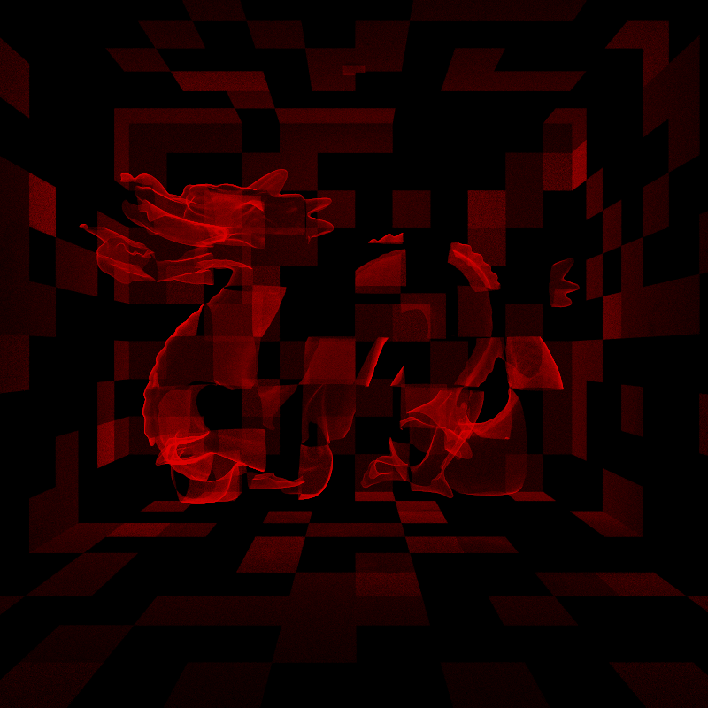 A visualization of the photon map, where only certain grids in the spatial hash grid are painted. Note that the grid size is largely exagerrated. You would NOT want to search with such a large radius
The spatial has grid is good for this application because it is very fast to build, simply requiring a hash and sort of a photon array. But theres more! From a GPU programming perspective, the spatial hash grid is a godsend, because its construction is incredibly parallel by nature. You can parallelize the hashing, you can parallelize the sort (like with a gpu radix sort), and at the end of it all, you have a sorted array of photons that have grid boxes stored consecutively in memory, allowing for coalesced memory access! No trees and no thread divergence!
However, SPPM does also share the harsh VRAM requirement that also plagued BDPT. You obviously need to store the photon map in VRAM, which is comparable in cost to storing the light path vertices in BDPT (though you usually need less data in a photon versus a light path vertex). However at the same, it is often neccesary to allocate two photon buffers, especially on GPU. This is because the best ways to sort the hashed photons, like the GPU radix sort, can’t really sort in place, so you constantly need to hold onto both an unsorted and sorted photon buffer.
The hardest part of implementing SPPM is just the data structure. You can probably tell, from the relative length of sections, that SPPM is way easier to implement that BDPT because you don’t need to do any MIS. But what if you did…
Vertex Connection and Merging 🔗
Vertex Connection and Merging (VCM) is what I would consider the final boss of established offline rendering. It is the most robust and versatile algorithm. It is essentially the combination of two existing global illumination algorithms: Bidirectional Path Tracing, and Stochastic Progressive Mapping, using Multiple Importance Sampling to weigh them together.
Earlier, we discussed how light path generation is remarkably similar to photon map generation. What VCM does is express photon mapping as an extension of the subpath expression of BDPT. In VCM, the BDPT part is expressed as Vertex Connections (VC), and the SPPM part is expressed as Vertex Merging (VM). Vertex Connections connect the vertices on the respective subpaths, just like BDPT.
Vertex Merging is re-expressed as merging light path vertices that are near eye path vertex together, that is also performed at EVERY bounce of the eye subpath, instead of just the first one, as is done with SPPM. From the previous explanation of SPPM, though, you may notice that this intuition kind of breaks the logic, because you can’t just merge two vertices, or say what is the likelihood of the light path vertex landing on the eye path vertex, since the math doesn’t support it. Merging is just a good descriptor of what you are doing in code, but not neccesarrily of what is actually happening mathematically. It’s better to think of it as extending the eye subpath by looking at a hypothetical light subpath, generated via the density estimation technique, and using that hypothetical light subpath to gain a contribution. The general intution is the same as in photon mapping. If I observe that around this point, generally light subpaths at this point are acting in a way that throws radiance in a direction, you can say that there is likely a light subpath precisely at the location of the eye subpath that acts similarly to the average of the light vertices near the query position.
In other words, instead of density estimating a radiance field, you estimate the density of light subpaths, and merge the end of the hypothetical subpath (that you know exists due to your density estimation!) with the end of your eye subpath. Importantly, this creates a path that looks just like a path generated by vertex connection (theres no micro-edge connecting a light subpath vertex and an eye subpath vertex), which allows it to be comapred with the other techniques using MIS.
The benefit of doing VCM is inherent in the use of the MIS. Since BDPT cannot efficiently sample SDS paths, and SPPM does it amazingly, but at the same time BDPT is overall much more consistent and importantly unbiased, VCM is able to use the best of both worlds, using VM more for SDS paths, while using VC more for the rest of the image. You can use VCM for any scene that SPPM or BDPT excels at, and it will do it as well, without needing to choose which one to use. Better yet, for mixed scenes where some parts are better rendered with one strategy and some are better with the other, VCM will always be better than either of the two.
VCM Implementation Details 🔗
The reason to merge BDPT and SPPM is because you can essentially get two data structures to gain samples with using one set of random walks. For each light path vertex you generate, you store it both as a light path vertex, and as a photon (separately). This also means that VCM is pretty rough on VRAM usage, since you have to manage both a light path buffer, and a photon buffer (or two, depending on implementation). You can’t store them together because you need them for vastly different memory access patterns and accessing one through the other would just be incredibly slow with respect memory access.
Other than that though, the math to integrate VM into a BDPT implementation (basically just VC) is not too hard, especially since the authors of VCM created a super helpful guide that gives you all of the formulas you need. Math-wise, it is just the addition of a term that describes the merging probability, which generally just slots in side by side with the other terms in the BDPT weight accumulation steps.